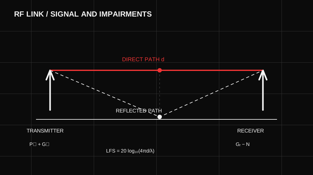
Radio investigations often begin with a tool name or a frequency label. A stronger starting point is a link model: where is energy launched, how does it propagate, what reaches the receiver, and what noise and interference compete with it? That model prevents two common errors: assuming a signal cannot be received outside a nominal coverage map, and assuming that hearing a signal means its content is readable.
This article develops a first-order link budget, then lists the conditions under which it stops being predictive. The interactive calculator is a teaching model for unobstructed free space; it is not a site survey or an authorization to intercept traffic.
From frequency to wavelength
An electromagnetic wave in vacuum travels at $c\approx299{,}792{,}458$ m/s. Frequency $f$ and wavelength $\lambda$ satisfy $\lambda=c/f$. At 2.4 GHz, the free-space wavelength is about 0.125 m. At 900 MHz it is about 0.333 m. Wavelength matters because antenna dimensions, diffraction around obstacles, and the size of the Fresnel zone scale with it.
An antenna is not simply a “signal amplifier.” It converts between guided energy and a radiated field and distributes sensitivity by direction and polarization. Gain in dBi compares radiation in a specified direction with an ideal isotropic radiator. A higher directional gain usually narrows the angular pattern; it does not create power. Effective aperture relates to gain as $A_e=G\lambda^2/(4\pi)$ when $G$ is linear, linking reception to wavelength and direction.
The far-field approximation itself has a boundary. A commonly used antenna criterion is $r\gtrsim 2D^2/\lambda$, where $D$ is the largest antenna dimension. Close to a large array, field geometry can differ from the plane-wave model used below. The criterion is a design rule, not a sharp physical wall.
Deriving the free-space loss term
For an isotropic source, power spreads over the area of a sphere, $4\pi d^2$. The power density at distance $d$ is $P_t/(4\pi d^2)$. Multiply by the receiving antenna’s effective aperture and include transmit and receive gains to obtain the Friis relation:
$$P_r=P_tG_tG_r\left(\frac{\lambda}{4\pi d}\right)^2$$
In decibels, the engineering form is $P_r(\mathrm{dBm})=P_t+G_t+G_r-L_{FS}-L_{other}$. The free-space basic transmission loss is:
$$L_{FS}=20\log_{10}!\left(\frac{4\pi d}{\lambda}\right)\ \mathrm{dB}$$
With frequency in MHz and distance in km, ITU-R P.525-5 gives the convenient approximation $L_{FS}\approx32.4+20\log_{10}f_{MHz}+20\log_{10}d_{km}$ dB. The unit convention is essential: inserting GHz or meters into that form without conversion produces a plausible-looking but wrong number.
For example, an unobstructed 2.4 GHz path over 1 km has approximately 100 dB free-space loss. With 20 dBm transmit power and 2 dBi antennas at both ends, the ideal received power is near $-76$ dBm before cable, polarization, obstruction, and fading losses. This is a budget illustration, not a prediction of a real street or building.
Radio link budget
Change frequency, distance, power, and gains. The estimate assumes far-field, unobstructed free-space propagation.
Keep the power reference straight
Transmit power at the radio connector is not the same as radiated power in a particular direction. Cable and connector loss occur before the antenna. The equivalent isotropically radiated power in that direction is $EIRP=P_t-L_t+G_t$ in dBm/dB units. A receiver then sees approximately
$$P_r=EIRP-L_{FS}+G_r-L_r-L_{pol}-L_{misc},$$
where $L_r$ is receive-side cable loss, $L_{pol}$ is polarization mismatch loss, and $L_{misc}$ collects other modeled losses. This accounting prevents an easy double count: if a device specification already gives EIRP, do not add transmitter antenna gain again. It also forces the measurement point into the notes. Was the 20 dBm read at the radio, inferred from configuration, or measured over the air?
An antenna pattern changes this budget with angle. A stated “8 dBi” is typically a peak or specified-direction value, not the gain toward every point around the antenna. Nulls and side lobes can make a nearby observer see less power than a farther observer in the main beam. A radio map that uses only distance and ignores orientation can therefore be confidently wrong.
Mismatch and losses at the feed
The Friis equation assumes power is transferred into and out of the antennas as modeled. Real feed lines, connectors, and antennas have impedance mismatch. A reflection coefficient $\Gamma$ gives a mismatch efficiency of $1-|\Gamma|^2$ for a simple port model; the corresponding mismatch loss is $-10\log_{10}(1-|\Gamma|^2)$ dB. This is one reason a long cable, poor connector, or badly matched antenna can erase the apparent benefit of an advertised gain figure.
Voltage standing-wave ratio (VSWR) is related to reflection magnitude by $VSWR=(1+|\Gamma|)/(1-|\Gamma|)$. It is a useful diagnostic of a feed, but it does not describe the antenna radiation pattern or the environment. A low VSWR does not guarantee that the antenna is pointed correctly, mounted clear of metal, or operating with the intended polarization.
Noise floor and usable signal
Received power alone does not tell us whether a receiver can decode a transmission. Thermal noise power is approximately $N=kTB$, where $k$ is Boltzmann’s constant, $T$ is system noise temperature, and $B$ is receiver bandwidth. In common dBm shorthand at roughly room temperature, $N\approx-174+10\log_{10}(B_{Hz})+NF$, where $NF$ is receiver noise figure in dB. The $-174$ term is an approximation tied to temperature, not a universal constant of every receiver. NIST defines the SI value of $k$.
At 20 MHz bandwidth, thermal noise is about $-101$ dBm before noise figure; a 5 dB noise figure moves the receiver floor near $-96$ dBm. The ideal $-76$ dBm example then has roughly 20 dB signal-to-noise ratio. Whether that is enough depends on modulation, coding, error target, interference, and implementation. In an actual assessment, measure rather than infer these from a marketing range claim.
The bandwidth term is not a minor adjustment. Double the effective noise bandwidth and thermal noise rises by about 3 dB, all else equal. Narrowing a receiver can improve the integrated noise floor, but only if the desired signal still fits in the passband. A strong out-of-band signal may also overload a real front end even when an ideal filter would reject it. This is why an SDR waterfall, a receiver sensitivity figure, and a packet decoder can disagree without any one of them being “broken.” They observe different stages of the receive chain.
Noise figure summarizes the receiver's added noise relative to an ideal input. It is not the same thing as an ambient noise measurement. In a crowded band, interference may dominate thermal noise. Signal-to-interference-plus-noise ratio, $SINR$, is then the more relevant quantity. In linear power units, $SINR=S/(I+N)$; subtracting dBm values directly inside that denominator is invalid. Convert to milliwatts, add, then convert back to dB if necessary.
Finally, decoding has a threshold shaped by modulation, coding, frame length, synchronization, and error correction. “I can see a peak” is evidence of energy. “I can recover symbols” is a stronger claim. “I can understand application data” is stronger again and may be blocked by encryption even at excellent RF quality.
What free space leaves out
The simple formula assumes clear line of sight, matched polarization, far-field conditions, and no significant reflections or absorption. Real links depart from it in several ways:
- Obstruction and diffraction. The first Fresnel zone has radius $r_1\approx\sqrt{\lambda d_1d_2/(d_1+d_2)}$ at a point with path distances $d_1$ and $d_2$. A visually clear centerline can still have poor Fresnel clearance.
- Multipath. A reflected wave may reinforce or cancel the direct wave depending on phase, delay, and position. A small receiver movement can change the result.
- Polarization mismatch. Antennas with different linear orientations lose coupled power; polarization can also change along a reflected path.
- Material and weather loss. Walls, foliage, terrain, rain, and gases add frequency-dependent attenuation.
- Interference. Another transmitter can dominate the link even when thermal noise is low.
ITU-R P.530 treats terrestrial line-of-sight design as a statistical problem involving diffraction, rain, multipath, and cross-polar effects. This is why a single free-space budget should be read as a baseline, not as a coverage guarantee.
At the midpoint of a 1 km, 2.4 GHz path, the first Fresnel-zone radius from the approximation above is about 5.6 m. A roof edge 2 m below the visual line between antennas still enters that zone. A common planning heuristic seeks substantial clearance of the first zone, often around 60%, but the exact effect depends on terrain and propagation. The calculation explains why “I can see the other antenna” is not a complete clearance test.
Multipath deserves an equally concrete picture. If a direct ray and a reflected ray arrive with similar amplitude but a phase difference near $\pi$, their electric fields can partly cancel. Move the antenna by a fraction of a wavelength and the phase relation changes. At 2.4 GHz, a wavelength is about 12.5 cm, so a desk-sized move can produce a conspicuous change. The receiver does not see separate neat rays; it sees their vector sum over frequency and time. Wideband signals may have frequency-selective fading, where some subcarriers are hit harder than others.
The security interpretation
RF range is a property of a transmitter, receiver, antennas, environment, and required signal quality together. It is not a fixed radius drawn around an access point. A more sensitive receiver or directional antenna can detect a signal beyond a client device’s practical service area. Conversely, a strong signal can be unusable because of interference or protocol protections.
Separate three questions during an authorized review:
- Can energy be detected? A spectrum observation answers only that some power is present in a band.
- Can a transmission be demodulated? This requires sufficient signal quality and a compatible physical layer.
- Can content or control be understood or changed? This depends on protocol design, authentication, encryption, keys, and implementation, not only RF power.
The same distinction matters defensively. A physical-layer map can identify unexpected reach, interference, or a weak link margin, but it cannot establish a cryptographic weakness. Document the frequency, bandwidth, antenna geometry, power assumptions, receiver, environment, and observed measurements before drawing a security conclusion.
Build a defensible measurement log
Before making a range claim, record the equipment chain: antenna model and orientation, cable length and loss, receiver model, gain setting, firmware or driver, measurement bandwidth, and any filtering. Record the clock and coordinate reference, plus whether the receiver was stationary or moving. A received-power number without gain settings and bandwidth is hard to compare across instruments.
Repeat observations at different positions and times. A single maximum reading overstates typical performance; a single null understates it. At a minimum, preserve the distribution or a few quantiles of measurements, not just the best value. Note obvious interferers and weather or obstruction changes. A link budget predicts a baseline; a measurement campaign tells you how often reality departs from it.
For a fixed link, calculate a fade margin: the gap between nominal received power and the receiver level required for the target error performance. If the nominal budget is $-76$ dBm and a receiver needs $-86$ dBm under the chosen mode, the nominal margin is 10 dB before additional losses and variability. That is not a 10 dB guarantee. It is room in the budget that may be consumed by fading, installation loss, rain, foliage, or interference. ITU-R P.530 treats several of these effects statistically for terrestrial line-of-sight systems.
Security questions the budget can and cannot answer
The budget can suggest where an unintended signal may be detectable, where a fixed link is fragile, and whether a directional antenna could plausibly change reception. It cannot tell you whether a network is authenticated, whether frames are replayable, whether keys are protected, or whether an application leaks data. Those are protocol and implementation questions. RF reach changes the set of places from which such questions might matter, but it does not answer them.
It is also easy to confuse a nominal transmit limit with a physical boundary. Regulatory limits and permitted tests depend on the country, band, service, and equipment. For research, use an authorized setup and document its configuration. The physics does not confer permission to transmit, jam, or capture someone else's communications.